Kalman filtering in FhSim

Fusion of measurements into the model simulation is useful for dynamically adapting the numeric simulation to e.g. real-world observations. FhSim facilitates state and parameter estimation using an Unscented Kalman Filter (UKF). Please read this documentation if you intend to use the built-in Kalman filtering in FhSim and/or are not familiar with Kalman filtering. To jump right to the core, see Implementing the KalmanObject.

Overview: Kalman filtering

This section will give a quick and dirty overview of the equations in a Kalman filter and UKF in particular. The reader is encouraged to consult resources elsewhere if a more in-depth introduction is sought.

Model description and measurements

Suppose we have a state vector \(x(t) \in \mathbb{R}^n\) with an ordinary differential equation on the form

\[\dot x = f(x,t) + w(t),\]

where \(w(t)\) is process noise. The system output \( y(t) \in \mathbb{R}^m\) is obtained at regular time points with period \(\Delta t\). The \(k\)th measurement occurs at \(t_k = t_0 + k\Delta t\) and is on the form

\[y_k := y(t_k) = h(x,t_k) + v(t_k),\]

where \(v(t)\) is measurement noise.

Covariance matrices

The objective of the Kalman filter is to provide an estimate of the state vector based on the available information. Information of relevance include initial conditions and the measurement sequence. Moreover, the Kalman filter exploits the statistical information about the process and measurement noise vectors together with the uncertainty of the state vector in determining the updated state vector. Let \( z \sim N(\mu,\Sigma) \) indicate that \(z \in \mathbb{R}^p\) is a multivariate vector with mean \(\mu\) and covariance matrix \(\Sigma \in \mathbb{R}^{p \times p}\), which is positive definite. Now, let

\begin{align*} w &\sim N(0,Q_c),\\ v &\sim N(0,R), \end{align*}

such that \(Q_c\) and \(R\) are the process and measurement covariance matrices, respectively. The diagonal terms of these matrices are the variance of the corresponding state derivative or measurement. The uncertainty of the state vector is taken as the covariance of the estimation error:

\[ P := E[(x - E[x]])(x - E[x])^T, \]

where \( E[\cdot]\) is the expectation operator. The estimation error covariance matrix \(P(t)\) (and the diagonal entries in particular) is a measure of how uncertain the state estimate is at a particular time point.

Note

The covariance \(Q_c\) above is given for the continuous-time case. In the discrete-time case the covariance matrix is given by the difference equation \(x_{k+1} = F(t_k,x_k) + w_k,\, w_k \sim N(0,Q)\). These to matrices are related by \(Q = \Delta t Q_c\). We will proceed by only mentioning the discrete variant, since this is used in the implementation.

The phases of a Kalman filter

The Kalman filter consists of three phases: initialization, time update, and measurement update. The last two phases are repeated for each new measurement, see diagram illustration.

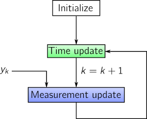
The three phases of Kalman filtering.

The initialization is done before the estimation itself begins. This includes setting the initial conditions of the state vector and other parameters, just as in a regular simulation in FhSim. The initial condition of the state vector \(\hat x(t_0) = \hat x_0\) is the best guess of the real state. With Kalman filtering the user also has to provide covariance matrices \(P(t_0),\,Q,\,R\).

The time update is an open-loop simulation from one time point \(t_{k-1}\) to \(t_k\), where a new measurement becomes available. For the Extended Kalman filter this is the solution to the initial value problem \( t \in [t_{k-1},t_k]\)

\[ \dot{\hat x}^-(t) = f(\hat x,t),\, \hat x(t_{k-1}) = \hat x_{k-1},\]

where \(\hat x_k^- =\hat x^-(t_k)\) is the so-called a priori estimate. This estimate is has not yet incorporated the measurement \(y_k\).

The estimation error covariance matrix also has to be updated. For the Extended Kalman filter this involves linearizing the system dynamics and solving a matrix differential equation, which includes of the previous time step's covariances \( P_{k-1}\) and \(Q\). Details will not be covered here.

Note

As we will see later, the a priori estimate is obtained in a different manner when using the UKF.

In the measurement phase the a priori estimates are updated by incorporating the information that the measurement \(y_k\) provides. The equations for this update are

\begin{align*} \hat x_k &= \hat x_k^- + K_k(y_k - \hat y_k)\\ P_k &= P_k^- - K_k P_y K_k^T, \end{align*}

where \(K_k\) is the Kalman gain matrix, which is based on the system uncertainties, and \( \hat y_k \) is the estimated measurement. \( \hat x_k \) is often called the a posteriori state estimate.

Unscented Kalman filter

The Extended Kalman filter (EKF) relies on first-order approximations of the mean and third-order approximations of the covariances when calculating the state estimates. These calculations require Jacobian information, which may be difficult to calculate/approximate accurately. The Unscented Kalman filter circumvent the Jacobian requirement by using so-called unscented transformations. This approach is based on two ideas:

1. A nonlinear transformation of a set of vectors are easier to compute than a nonlinear transformation of a whole probability density function (pdf).
2. It is possible to find a deterministic set of vectors that approximates a given pdf.

When the unscented transformations are used to propagate the means and covariances instead of its linearized counterparts of the EKF, it is called the Unscented Kalman filter. The method enjoys the benefit of tackling highly nonlinear systems with discontinuities better than for instance the EKF. This approach was first proposed in Julier, S. J., Uhlmann, J. K., and Durrant-Whyte, H. F. (1995). "A new approach for filtering nonlinear systems". In American Control Conference, pages 1628-1632, Seattle, Washington, USA.

The unscented transformation

An unscented transformation is basically the function evaluation of a set of input vectors through a nonlinear function. The outputs of these function evaluations are used to approximate the statistical properties, such as mean and covariance, of the nonlinear transformation. By appropriately choosing the input vectors and the weighting when combining the outputs, we obtain an approximation of the probability density function of the transformation at hand.

Suppose that we have a nonlinear function \( y: R^n \to R^n\), whose domain has known mean and covariance:

\begin{align*} y &= h(x)\\ x &\sim N(\hat x, P_x). \end{align*}

Let \(\{x^{(i)}\}_0^{2n}\) be a sequence of carefully chosen sigma points. We perform a nonlinear transformation \(h(\cdot)\) of all these points to get a mapped sequence \(\{y^{(i)}\}_0^{2n}\). Weighted sums and sample covariance of these outputs provide us with an approximated mean and covariance of the mapping \( h(\cdot)\), namely \( \hat y\) and \(\hat P_y\). This procedure is illustrated for a two-dimensional mapping in the figure below.

The mapping of five sigma points for a two-dimensional mapping. The ellipsoids illustrate level sets of the corresponding covariance matrices.

Note

There are in general two nonlinear mappings in the system to be estimated, namely \(f(\cdot)\) and \(h(\cdot)\) in the right-hand-side of the differential equation and measurement function, respectively. The unscented Kalman filter then has to solve an initial value problem (IVP) for each perturbation (sigma point) of the state vector. The resulting sequence of a priori state vectors is used to approximate the mean and covariance. For each of these propagated sigma points the measurement mapping is also calculated. Since \(2n+1\) IVPs have to be solved for a state vector of size \(n\), the calculation time may be high if \(n\) is large. There are also steps related to carefully choosing sigma points that are costly, so the UKF algorithm does not scale particularly well with state dimension.

Implementation in FhSim

In FhSim the UKF is implemented based on the publication http://www.dx.doi.org/10.1109/ICASSP.2001.940586. Please consult this publication for details on the equations involved. We have implemented both the normal and the square root variant, but due to numerical issues (or implementation errors) with the latter, we currently use the normal one.

The Kalman filter implementation make use of three central classes in FhSim: CKalmanIntegrator, estimator::KalmanFilter, and KalmanObject. In addition, some supporting data structures are used.

CKalmanIntegrator utilizes a user-specified fixed-step COdeSolver to step the state forward in time. It also assembles covariance matrices and measurement vector contributions from each KalmanObject. This information is used by the estimator::KalmanFilter (and its child estimator::UKF) to solve the Kalman filter equations and update the state estimate vector and other relevant data structures as described in the above mentioned paper. The two most costly operations in the filter are to simulate the ensemble of sigma points forward in time and the solution to a matrix square root. The ensemble update involves the solution to \(2n+1\) IVPs. In contrast, a pure simulation only needs to solve one IVP at any given time. Large-scale systems are thus expected to struggle for real-time performance (Note: Profiling of the Kalman filter may reveal sources for improvement).

The user usually only has to deal with the KalmanObject interface to use the Kalman filter functionality in their own simulations.

How to use Kalman filtering in FhSim

Suppose you want to estimate some process using a Kalman filter. If you already have implemented a SimObject, you are in luck, because then you only have to inherit from this object in addition to the KalmanObject interface. In broad strokes, once a SimObject has been extended with the KalmanObject interface, the input file for a KalmanObject is not very different from a regular SimObject. Only some new connections and/or input parameters may need to be defined.

The implementation defines a KalmanObject interface class. This class declares several virtual functions that need to be defined in order to enable Kalman filtering. We provide two examples to get you started.

1. Example: Simple pendulum
2. Case study: A sphere attached to a cable submerged in water

The pendulum example gives you a cut-to-the-bone introduction of what you need to do to get started, whereas the case study is a bit more involved, providing some more guidelines and details on how to use Kalman filtering in your project, faced with some additional challenges.

Case study: A sphere attached to a cable submerged in water

Suppose we have a cable connected to a fixed point in one end and a sphere mass in the other end, both points submerged in water. The setup is under the influence of gravity, buoyancy, and some unknown, slowly-varying current. Every \(\Delta t\) seconds a noisy measurement of the sphere position is obtained. Our objective is to estimate the cable's state vector and the water current. We proceed by modeling the problem as a simple hydrodynamic cable and ball, each component modeled in their own SimObject.

Let the inertial reference frame be fixed to north, east, and down directions with coordinates ordered as \((N,E,D)\). Define \(v_c(t) \in \mathbb{R}^3\) as the slowly-varying uniform current.

Case study: Hydrodynamic ball model

Define \(p(t) \in \mathbb{R}^3\) and \(v(t) \in \mathbb{R}^3\) as position and velocity of the ball, respectively. The ordinary differential equations for the hydrodynamic ball are

\begin{align*} \dot p &= v,\\ \dot v &= \frac{F(p,v,t)}{m}, \end{align*}

where \(F\) is the force acting on the ball and \(m\) is the ball's mass. The forces acting on the ball are gravity, buoyancy \(B\), drag \(D\), and other external forces: \(F(p,v,t) = mg - B + D + f_{ext}(p,v,t)\), where \(g = (0,0,9.81)\). We use that the ball volume is \(\frac{4}{3}\pi r^3\) and assume that the ball is completely submerged, so \( B = \frac{\rho_w}{\rho_b}mg\), with \(\rho_w,\,\rho_b\) being the water and ball density, respectively. The drag on the ball is modelled as Morison drag \( D = -0.5 \rho_w \pi r^2 C_d (v-v_c)\|v-v_c\|_2\), where \(r\) is the ball radius and \(C_d\) is the drag coefficient (the latter is set to \(0.5\)). After simplifying the equations we arrive at the following force function

\[ F = mg\left(1 - \frac{\rho_w}{\rho_b}\right) - m\frac{3C_d}{8r}\frac{\rho_w}{\rho_b}v_r \|v_r\|_2 + f_{ext}(p,v,t), \]

where \(v_r := v - v_c\) is the relative current.

Define \( x_b(t) := [p^T\, v^T]^T \in \mathbb R^6\) as the state vector for the ball. The compact description for the ball dynamics is

\begin{align*} \dot x_b &= f_b(x_b,t),\\ y_b(t) &= p(t) + v(t), \end{align*}

where \(y_b(t)\) is the noisy measurement of the ball's position.

Case study: Hydrodynamic cable model

We model a simple mass-lumped cable that consists of point masses connected by spring and damper forces. Like the ball, the cable is under the influence of gravity, buoyancy, and Morison drag. The characteristics of the cable are given in the table below.

Description	Symbol	Numeric value (if const.)
Length	\(L\)	-
Diameter	\(d\)	-
Density	\(\rho_c\)	-
Mass	\(M\)	\(\rho_c \pi \left(\frac{d}{2}\right)^2 L\)
Elastic modulus	\(E\)	-
Cross-section drag coef.	\(C_d\)	1.1
Streamlined drag coef.	\(C_t\)	0.1

We discretize the cable into \(n+1\) uniform line segments, so that there are \(n\) point masses excluding the end points. Each point has mass \(m_i = \frac{M}{n}\). Let \( i \in \{1,2,\dots,n\} =: \mathbb{I}_n\) be the indices of the points. The indices \(i = 0\) and \(i = n+1\) are the end points. For each \(i \in \mathbb{I}_n\) let \(p_i(t),v_i(t) \in \mathbb R^3\) be the position and velocity with dynamics

\begin{align*} \dot p_i &= v_i,\\ \dot v_i &= \frac{F_i(p_{i-1},p_i,p_{i+1},v_i,t)}{m}, \end{align*}

where \(F_i\) is the forces acting on the \(i\)th point mass. The forces are

\[ F_i = m_ig\left(1 - \frac{\rho_w}{\rho_c}\right) + D_i + \Lambda_i + \Delta_i, \]

where \(\rho_w\) is water density, \(D_i\) is drag, \(\Lambda_i\) is spring forces, and \(\Delta_i\) is damper forces. In the following we will define the drag, spring, and damper forces.

Drag forces

Each point mass has two line segments connected to it. From each of these two line segments there will be a contribution to the drag that acts on the point. We take half a line segment's length and calculate the drag on this cylinder. Let us continue by defining some expressions that make the exposition simpler. Let \(k,l \in \mathbb I_n \cap \{0,n+1\}, k\neq l\).

\begin{align*} \bar p (k,l) &:= \frac{p_l - p_k}{\|p_l - p_k\|_2},\\ v(k,v_c) &:= v_k - v_c,\\ v_{k,l}^\| &:= \left(v(k,v_c)\cdot \bar p(k,l)\right)\bar p(k,l),\\ v_{k,l}^\perp &:= v(k,v_c) - v_{k,l}^\|, \end{align*}

where \(v_c(t) \in \mathbb R^3\) is the water current and \(\cdot\) is the dot product. \(\bar p\) is the unit vector pointing from \( p_k\) to \(p_l\). \( v(k,v_c)\) is the velocity of \(p_k\) relative to the current, whereas \(v_{k,l}^\|\) and \(v_{k,l}^\perp\) are the decomposition into a velocity parallel to and perpendicular to the corresponding line segment, respectively.

The drag on line segment \((k,l)\) acting on point \(k\) is

\[ D(k,l) = -\frac{1}{2}\rho_w \underbrace{d 0.5\|p_l - p_k\|_2}_{A} \|v(k,v_c)\|_2\left(C_d v_{k,l}^\perp + C_t v_{k,l}^\| \right). \]

The total drag on point \(i \in \mathbb I_n\) is

\[ D_i = D(i,i+1) + D(i,i-1). \]

Spring forces

The spring forces acting on a point mass come from the line segments connected to the neighboring points. The relaxed length of line segment \((k,l)\) is \( L_0(k,l) = \frac{L}{n+1} := L_0\). We assume linear spring forces under extension only (no compression forces). The spring force acting on point \(k\) due to line segment \((k,l)\) is

\[ \Lambda(k,l) = \begin{cases} \overbrace{E\pi \frac{d^2}{4} \frac{1}{L_0}}^{\lambda}\left(\|p_l - p_k\|_2 - L_0 \right)\bar p(k,l) &\mbox{if } \|p_l - p_k\|_2 \geq L_0\\ 0 & \mbox{otherwise } \end{cases} \]

The spring forces acting on point \(i \in \mathbb I_n\) are

\[ \Lambda_i = \Lambda(i,i+1) + \Lambda(i,i-1). \]

Damper forces

The damping forces on a point in the cable also depend on the neighboring points. We denote the damping on point \(k\) from point \(l\) as

\[ \Delta(k,l) = 2\sqrt{\lambda m_k}\left((v_l - v_k) \cdot \bar p(k,l) \right)\bar p(k,l), \]

where \( k \) was defined when discussing spring forces.

The damping forces acting on point \(i\in \mathbb I_n\) are

\[ \Delta_i= \Delta(i,i+1) + \Delta(i,i-1). \]

Compact cable description

We have now described all forces acting on the cable. Putting it all together and detailing the compact description are outside the scope of this case study. We simply state that there exist such an equation. Define \( x_c(t) = [p_1^T\, v_1^T\, \cdots\, p_n^T\, v_n^T]^T \in \mathbb R^{6n}\) as the cable state vector with compact description

\begin{align*} \dot x_c &= f_c(x_c,t), \end{align*}

where the end points and water current are considered time-varying expressions.

Case study: Input files

Simulator setup

Both the hydrodynamic ball and cable have been implemented as SimObjects. Their documentation and can be found in the fhsim_base under Example/HydroBall and Example/HydroCable. We assume that the setup is under the influence of a current, which consists of sine-wave with bias in north direction, and constant current in east and down directions.

\[ v_c(t) = \begin{bmatrix}a\sin(\omega t) + b\\c\\d\end{bmatrix}, \]

where \(a,\, \omega,\, b,\, c,\, d\) are sine-wave amplitude, angular velocity, bias, and constants, respectively.

We use the following input files for simulation of a ball connected to a cable.

Simulation.xml:

<Contents>
  <OBJECTS>
    <Lib
        LibName = "fhsim_base"
        SimObject = "Src/Sine"
        Name = "NorthCurrent"
        PortWidth = "1"
        PhaseRad = "0"
        PeriodS = "200"
        StartTime = "0"
        StopTime = "-1"
        Bias = "0.7"
        Amplitude = "0.3"
    />
 
    <Lib
        LibName = "fhsim_base"
        SimObject = "Signal/Mux"
        Name = "Current"
        NumInput = "3"
        PortWidth = "3"
        InPortWidth1 = "1"
        InPortWidth2 = "1"
        InPortWidth3 = "1"
    />
 
    <Lib
        LibName = "fhsim_base"
        SimObject = "Example/HydroBall"
        Name = "Ball"
        Radius = "1.0"
        Density = "1100"
    />
    <Lib
        LibName = "fhsim_base"
        SimObject = "Example/HydroCable"
        Name = "Cable"
        Diameter = "0.02"
        Density = "2000"
        Modulus = "20"
        Length = "20"
        InternalPoints = "7"
    />
  </OBJECTS>
 
  <INTERCONNECTIONS>
    <Connection
        Ball.ExternForce = "Cable.ForceB"
        Ball.Current     = "Current.Out"
 
        Current.In1      = "NorthCurrent.Out"
        Current.In2      = "0.5"
        Current.In3      = "0.1"
    />
 
    <Connection
        Cable.PositionA = "0,0,0"
        Cable.PositionB = "Ball.Position"
        Cable.VelocityA = "0,0,0"
        Cable.VelocityB = "Ball.Velocity"
        Cable.Current   = "Current.Out"
    />
  </INTERCONNECTIONS>
 
  <INITIALIZATION>
    <InitialCondition
        Ball.Position = "0,6.15,18.9"
        Ball.Velocity = "0,0,0"
    />
  </INITIALIZATION>
 
  <INTEGRATION>
    <Engine
        IntegratorMethod="0"
        NumCores="1"
        TOutput="0, 0:1e-1:Inf, 1000"
        stepsize ="2e-4"
        FileOutput="objects:ports"
    />
 
  </INTEGRATION>
</Contents>

Now, suppose the simulation described in A sphere attached to a cable submerged in water in the section above is "a real-world process" and we do not know neither the current, nor the states of the ball or cable. We do, however, get a noisy measurement of the ball's position every \(\Delta t \) seconds. Our objective is to estimate the cable's state vector and the water current.

The simulator setup is as follows. We start a FhSim process and denote this the real-world simulation. Usually, information about the real-world process is collected through various sensors and peripheral devices with various sampling rates and noise. To mimic this behavior we:

• use the Signal/Samplifier SimObject to do a sample and hold with artificially added noise to the ball position.
• employ FhSim's Data Distribution Service (DDS) interface to collect and send information periodically.

We add the following code snippet at appropriate locations in Simulation.xml above (consult documentation for respective SimObjects for details)

<Lib
    LibName            = "fhsim_base"
    SimObject          = "Signal/Samplifier"
    Name               = "Sample"
    PortWidth          = "1"
    NoiseSeed          = "42"
    Tags               = "NorthEastDown"
    SamplingPeriod1    = ".1, .1, .1"
    NoiseBias1         = "0, 0, 0"
    NoiseStdDev1       = "0.15, 0.15, 0.05"
/>
 
<Lib LibName    = "fhsim_extras"
     SimObject  = "Connection/DdsWriter"
     Name       = "Send"
     Partition  = "FhSimExternal"
     Topic      = "CableMeasure"
     DdsRoot    = "../lib"
     DdsConfigFile = "../resources/ospl.xml"
     ForceDdsEnv = "0"
     PortWidth  = "1"
     ArrayIDs   = "0"
     PortSizes  = "3"
     SamplingPeriods = "0.1"
     />
 
<Connection
    Sample.In1      = "Ball.Position"
    Send.In1        = "Sample.NorthEastDown"
/>

Simulation.xml now simulates the real world process, obtains measurements at regular intervals, and sends them via DDS to be accessed by the estimator. The estimator, which is another FhSim process, employs KalmanObjects and incorporates the received measurements of the simulated real world. We continue by first describing the estimator setup and then detailing the necessary KalmanObject implementations.

Estimator setup

When estimating the process at hand we need mathematical descriptions of the objects involved. Luckily, we already have implemented SimObjects that capture most of the phenomena at hand. What we do not know, though, is the time-varying current. A common assumption when estimating parameters is to assume that they are constant or slowly-varying. In such a case, one can describe the process with "zero-dynamics" as follows. Suppose \( p(t) \in \mathbb{R}^m\) is an parameter vector with dynamics

\[ \dot p = 0 + w_p(t), \]

where \(w_p(t)\) is process noise. The initial conditions for this differential equation are the best guesses of the parameters. We use this description for the current in the estimator.

The involved SimObjects have been extended to KalmanObjects and the file below serves as the input file for the estimator.

Estimation.xml:

<Contents>
  <OBJECTS>
    <Lib
        LibName = "fhsim_base"
        SimObject = "Kalman/ZeroDynamics"
        Name = "Current"
        Dimension = "3"
        P0 = "5e-2,5e-2,1e-4"
        Q = "1e-4,1e-4,1e-5"
    />
 
    <Lib
        LibName = "fhsim_base"
        SimObject = "Kalman/Example/HydroBall"
        Name = "Ball"
        Radius = "1.0"
        Density = "1100"
 
        MeasurementNoise     = "1"
        PositionUncertainty  = "5e-4"
        VelocityUncertainty  = "1e-6"
        InitialDiagP         = "1e-3,1e-3,1e-3,1e-3,1e-3,1e-3"
    />
 
    <Lib
        LibName = "fhsim_base"
        SimObject = "Kalman/Example/HydroCable"
        Name = "Cable"
        Diameter = "0.02"
        Density = "2000"
        Modulus = "20"
        Length = "20"
        InternalPoints = "2"
 
        ElementPositionUncertainty  = "5e-4"
        ElementVelocityUncertainty  = "1e-6"
        ElementInitialDiagP         = "1e-3,1e-3,1e-3,1e-3,1e-3,1e-3"
    />
 
    <Lib LibName    = "fhsim_extras"
         SimObject  = "Connection/DdsReader"
         Name       = "Receive"
         Partition  = "FhSimExternal"
         Topic      = "CableMeasure"
         DdsRoot    = "../lib"
         DdsConfigFile = "../resources/ospl.xml"
         ForceDdsEnv = "1"
         InitializationTimeout = "2000"
         PortWidth  = "1"
         Tags       = "Out"
         DefaultOut = "0,0,0"
         ArrayIDs   = "0"
         PortSizes  = "3"
         />
 
  </OBJECTS>
 
  <INTERCONNECTIONS>
 
    <Connection
        Ball.ExternForce = "Cable.ForceB"
        Ball.Current     = "Current.State"
    />
 
    <Connection
        Cable.PositionA = "0,0,0"
        Cable.PositionB = "Ball.Position"
        Cable.VelocityA = "0,0,0"
        Cable.VelocityB = "Ball.Velocity"
        Cable.Current   = "Current.State"
    />
 
    <Connection
        Ball.MeasuredPosition = "Receive.Out"
    />
 
    </INTERCONNECTIONS>
 
  <INITIALIZATION>
    <InitialCondition
        Ball.Position = "0,19,0"
        Ball.Velocity = "0,0,0"
        Current.State = "0,0,0"
    />
  </INITIALIZATION>
 
  <INTEGRATION>
    <Engine
        IntegratorMethod="0"
        NumCores="1"
        TOutput="0, 0:1e-1:Inf, 150"
        stepsize ="2e-4"
        HMin="0.5"
        FileOutput="objects:ports"
    />
 
  </INTEGRATION>
</Contents>

The contents of Estimator.xml is quite similar to Simulator.xml, with some extensions.

• We use instead a Connection/DDSReader to receive the information that the Connection/DDSWriter sends.
• The cable has fewer internal elements.
• Each KalmanObject has additional parameters that must be defined.
• Kalman/Example/HydroBall has a new input port, namely a measurement of its position.

Note

Measurements are incorporated at major time steps \(\Delta t > 0\) only. \(\Delta t\) is usually much larger than the step size of the integrator. It is specified in the XML-element INTEGRATION::Engine as the parameter HMin in seconds. In Estimator.xml above, the major time step is 0.5 s, so there are 2 500 integrator steps per measurement update. The major time step \( \Delta t\) must be a integer multiple of the step size (if not, this will be enforces).

Warning

Only fixed-step integrators are supported when using KalmanObjects.

HydroBall with KalmanObject extension

Let's proceed with the Kalman extension of the Example/HydroBall. Consider below the declaration of KalmanHydroBall that has the KalmanObject extension.

#include "KalmanObject.h"
 
class KalmanHydroBall : public HydroBall, public KalmanObject{
public:
  KalmanHydroBall(const std::string& simObjectName, ISimObjectCreator* const creator);
  estimator::Matrix GetCovarianceP0();
  estimator::Matrix GetProcessNoiseQ();
  estimator::Matrix GetMeasurementNoiseR();
  estimator::Vector ExpectedMeasurementOutput(const double T, const double* const X);
  estimator::Vector ActualMeasurementOutput(const double T,, const double* const X);
  unsigned int GetNumMeasurements();
 
protected:
  ISignalPort* m_PositionMeasurement;
  double m_MeasurementNoise;
  double m_PositionUncertainty;
  double m_VelocityUncertainty;
  double m_InitialP[6];
 
};

Notice that the class inherits from both HydroBall and KalmanObject, so we need to define some virtual fuctions.

Note

We make heavily use of the Eigen library for vector and matrix operations. The type definitions estimator::Vector and estimator::Matrix are, respectively, dynamically sized double vectors and matrices from the Eigen library. Readers unfamiliar with this library should consult its documentation Eigen::GettingStarted and Eigen::QuickReferenceGuide.

Below we have included the definition for each function of KalmanHydroBall. We will not explain every line of code, since it is (by some) deemed self-explanatory.

Implementation of Kalman/Example/HydroBall:

// The constructor calls the constructor for HydroBall and adds a new input port. Some new parameters are also fetched from the input file.
KalmanHydroBall::KalmanHydroBall(const std::string& simObjectName, ISimObjectCreator* const creator)
  : HydroBall(simObjectName, creator)
{
  creator->AddInport("MeasuredPosition", 3, &m_PositionMeasurement);
  creator->GetDoubleParam("MeasurementNoise", &m_MeasurementNoise);
  creator->GetDoubleParam("PositionUncertainty", &m_PositionUncertainty);
  creator->GetDoubleParam("VelocityUncertainty", &m_VelocityUncertainty);
  creator->GetDoubleParamArray("InitialDiagP", m_InitialP, 6);
}
 
// This function creates the P0 from the given input parameters and returns it as a 6x6 matrix.
estimator::Matrix KalmanHydroBall::GetCovarianceP0()
{
  estimator::Vector diagP0(6);
  diagP0 <<
    m_InitialP[0],     m_InitialP[1],     m_InitialP[2],
    m_InitialP[3],     m_InitialP[4],     m_InitialP[5];
  return Eigen::DiagonalMatrix<double,Eigen::Dynamic>(diagP0);
}
 
// 6x6 process noise matrix Q.
estimator::Matrix KalmanHydroBall::GetProcessNoiseQ()
{
  using namespace estimator;
  Vector diagQ_pos = m_PositionUncertainty*Vector::Ones(3);
  Vector diagQ_vel = m_VelocityUncertainty*Vector::Ones(3);
  Vector diagQ(6);
  diagQ << diagQ_pos, diagQ_vel;
  return Eigen::DiagonalMatrix<double,Eigen::Dynamic>(diagQ);
}
 
// 3x3 measurement noise matrix R.
estimator::Matrix KalmanHydroBall::GetMeasurementNoiseR()
{
  estimator::Vector diagR = m_MeasurementNoise*estimator::Vector::Ones(3);
  return Eigen::DiagonalMatrix<double,Eigen::Dynamic>(diagR);
}
 
// Returns the 3D estimated position of the ball.
// Note that cached functions evaluations such as Position(T,X) must NOT be used.
estimator::Vector KalmanHydroBall::ExpectedMeasurementOutput(const double T, const double* const X)
{
  estimator::Vector ret(3);
  ret << X[m_PositionIndex], X[m_PositionIndex+1], X[m_PositionIndex+2];
  return ret;
}
 
// Gets the position measurement of the ball.
estimator::Vector KalmanHydroBall::ActualMeasurementOutput(const double T, const double* const X)
{
  const double* y = m_PositionMeasurement->GetPortValue(T,X);
  estimator::Vector ret(3);
  ret << y[0], y[1], y[2];
  return ret;
}
 
// Returns the dimension of this object's measurement vector.
unsigned int KalmanHydroBall::GetNumMeasurements()
{
  return 3;
}

Warning

The implementer must ensure that the columns/rows in the covariance matrices are arranged in the same order as the state or output variable vector. Above, the position state variables were created before velocity state variables (order of call to AddState(.) in the constructor of HydroBall), hence elements for position uncertainty comes before velocity uncertainty.

After following fs-page-create-simobject-or-library, KalmanHydroBall is accessible for use with FhSim.

HydroCable with KalmanObject extension

The KalmanHydroCable is implemented in a similar fashion as the KalmanHydroBall, so the code will not be presented here. Some code will be given to highlight important points.

Excerpt of Kalman/Example/HydroCable:

#include <unsupported/Eigen/KroneckerProduct> // included to allow block-diagonal replication of matrix.
 
// P0 consists of block matrices for each internal point in the cable
estimator::Matrix KalmanHydroCable::GetCovarianceP0()
{
  using namespace estimator;
  Vector diagP0(6);
  diagP0 <<
    m_InitialP[0],     m_InitialP[1],     m_InitialP[2],
    m_InitialP[3],     m_InitialP[4],     m_InitialP[5];
 
  Matrix P0i = Eigen::DiagonalMatrix<double,Eigen::Dynamic>(diagP0);
 
  int m = m_NumPoints; // number of internal points
  Matrix I = Matrix::Identity(m,m); // Diagonal matrix of ones.
 
  // P0i is multiplied with each scalar in I, resulting in a block diagonal matrix of P0i's (dimension: m6 x m6)
  Matrix P0 = Eigen::kroneckerProduct(P0i,I);
 
  return P0;
}
 
// All functions must be implemented, like below, even if there are no measurements in the object.
estimator::Vector KalmanHydroCable::ExpectedMeasurementOutput(const double T, const double* const X)
{
  return estimator::Vector();
}

When the number of internal states depends on input parameters, the implementer must take care so that the dimensions of belonging matrices in KalmanObject scales accordingly.

ZeroDynamics

One can of course implement a SimObject with KalmanObject interface directly, where both the SimObject and KalmanObject interface are implemented simultaneously:

class ZeroDynamics : public SimObject, public KalmanObject{
public:
  ZeroDynamics(const std::string& simObjectName, ISimObjectCreator* const creator);
 
  // SimObject functions
  void OdeFcn(const double T, const double* const X, double* const XDot, const bool IsMajorTimeStep);
  void InitialConditionSetup(const double T, const double* const currentIC, double* const updatedIC, ISimObjectCreator* const creator);
 
#ifdef FH_VISUALIZATION
  void RenderInit(Ogre::Root* const ogreRoot, ISimObjectCreator* const creator){};
  void RenderUpdate(const double T, const double* const X){};
#endif
 
  // KalmanObject functions
  estimator::Matrix GetCovarianceP0();
  estimator::Matrix GetProcessNoiseQ();
  estimator::Matrix GetMeasurementNoiseR(){ return estimator::Matrix(); }
  estimator::Vector ExpectedMeasurementOutput(const double T, const double* const X){ return estimator::Vector(); }
  estimator::Vector ActualMeasurementOutput(const double T, const double* const X){ return estimator::Vector(); }
  unsigned int GetNumMeasurements(){ return 0; }
 
protected:
  void SetOutputPortValues(const double T, const double* const X);
  const double * Output( const double T, const double * const X);
 
  ICommonComputation* m_SetOutputPortValues;
  int m_StateIndex, m_NoStates;
  std::unique_ptr<double[]> m_State;
  std::unique_ptr<double[]> m_P0, m_Q;
};

See Running the simulator and estimator example(s) on how to run the code.

Case Study: Results

The above example has been run and below you can se the measured and estimated position of the ball. You can also see the true and estimated current in the three lower subplots.

Using position measurements of the ball, we are able to approximate the current that influences the displacement of the ball. The estimates are not very good, and there may be several reasons for this:

• We have artificially added white noise to the position measurement, which influence the quality of the estimates.
• Tuning the Kalman parameters (Q, R) for each KalmanObject is a tedious and difficult task. Better tuning may give better performance, and vice versa.
• The information from the measurement may not be rich enough to observe the real state. This may be particularly true for the z-component of the current, since we see a bias in the estimate.

It should be pointed out that we use identical numerical model descriptions for the simulator and estimator. This is not the case when filtering real-world measurements, and may be reflected in the estimator performance.

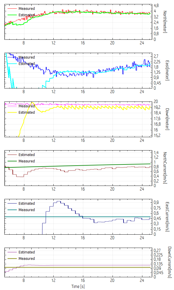
Measured and Estimated ball position and current.

Example: Simple pendulum

Consider a simple pendulum with angle \(\theta\) with respect to the z-axis of a north, east, and down reference frame, and angular velocity \(\omega\)

\begin{align*} \dot \theta &= \omega\\ \dot \omega &= -\frac{g}{l}\sin \theta, \end{align*}

where \(g\) is standard gravity and \(l\) is pendulum arm length.

Example: KalmanObject declaration

Suppose you want to estimate its movement, given an angle measurement every \(\Delta t \) seconds. The pendulum is implemented in FhSim as the class Pendulum (Example/Pendulum). To implement the KalmanObject interface on this class, consider the following class declaration, which inherits from both Pendulum and KalmanObject:

#include "KalmanObject.h"
 
class KalmanPendulum: public Pendulum, public KalmanObject{
public:
  Pendulum(const std::string& simObjectName, ISimObjectCreator* const creator);
  estimator::Matrix GetCovarianceP0();
  estimator::Matrix GetProcessNoiseQ();
  estimator::Matrix GetMeasurementNoiseR();
  estimator::Vector ExpectedMeasurementOutput(const double T, const double* const X);
  estimator::Vector ActualMeasurementOutput(const double T,, const double* const X);
  unsigned int GetNumMeasurements();
 
protected:
  ISignalPort* m_AngleMeasurement;
  double m_MeasurementNoise;
  double m_AngleUncertainty;
  double m_AngularVelocityUncertainty;
  double m_InitialP[2];
 
};

This code shows the declarations of the virtual function from the KalmanObject interface that must be implemented.

Example: KalmanObject definitions

The corresponding definitions for the above code is

// Constructor calling the Pendulum constructor and retrieving new parameters for the Kalman covariance matrices.
KalmanPendulum::KalmanPendulum(const std::string& simObjectName, ISimObjectCreator* const creator)
  : Pendulum(simObjectName, creator)
{
  creator->GetDoubleParam("AngleNoise", &m_AngleUncertainty);
  creator->GetDoubleParam("AngularVelocityNoise", &m_AngularVelocityUncertainty);
  creator->GetDoubleParam("MeasurementNoise", &m_MeasurementNoise);
  creator->GetDoubleParamArray("InitialP",m_InitialP, 2);
 
  creator->AddInport("Angle", 1, &m_AngleMeasurement); // This is a new input, which is angle measurement.
}
 
// Specifies a diagonal initial estimation error covariance matrix.
estimator::Matrix KalmanPendulum::GetCovarianceP0()
{
  estimator::Matrix ret(2,2);
  ret <<
    m_InitialP[0],0,
    0,m_InitialP[1];
  return ret;
}
 
// Diagonal process noise matrix Q.
estimator::Matrix KalmanPendulum::GetProcessNoiseQ()
{
  estimator::Matrix ret(2,2);
  ret <<
    m_AngleUncertainty,0,
    0,m_AngularVelocityUncertainty;
  return ret;
}
 
// Measurement noise matrix R (happens to be scalar).
estimator::Matrix KalmanPendulum::GetMeasurementNoiseR()
{
  estimator::Matrix ret(1,1);
  ret(0,0) = m_MeasurementNoise;
  return ret;
}
 
// Actual measurement retrieved from the port function. Angle.
estimator::Vector KalmanPendulum::ActualMeasurementOutput(const double T, const double* const X)
{
  const double* y = m_AngleMeasurement->GetPortValue(T,X);
  estimator::Vector ret(1);
  ret << m_AngleMeasurement->GetPortValue(T,X)[0];
  return ret;
}
 
// Expected measurement given from the state estimate vector (angle)
estimator::Vector KalmanPendulum::ExpectedMeasurementOutput(const double T, const double* const X)
{
  estimator::Vector ret(1);
  ret << X[m_AngleIndex];
  return ret;
}
 
// Returns the dimension of the measurement vector.
unsigned int KalmanPendulum::GetNumMeasurements()
{
  return 1;
}

Example: Input files

To run a simulation using this code, we define two input files: one for a simulator, which emulates the real world, and an estimator, which tries to mimic the real world, given angle measurements on a regular interval. The measurement is transmitted using a Data Distributive Service (DDS) SimObject.

The input file for Simulator.xml is

<Contents>
  <OBJECTS>
    <Lib
        LibName = "fhsim_base"
        SimObject = "Example/Pendulum"
        Name = "Pen"
        Length = "3"
    />
 
    <Lib LibName    = "fhsim_extras"
         SimObject  = "Connection/DdsWriter"
         Name       = "Send"
         Partition  = "FhSimExternal"
         Topic      = "PhysicalEntity"
         DdsRoot    = "../lib"
         DdsConfigFile = "../resources/ospl.xml"
         ForceDdsEnv = "0"
         PortWidth  = "1"
         ArrayIDs   = "0"
         PortSizes  = "1"
         SamplingPeriods = "0.1"
         />
  </OBJECTS>
 
  <INTERCONNECTIONS>
    <Connection
        Send.In1 = "Pen.Angle"
    />
  </INTERCONNECTIONS>
 
  <INITIALIZATION>
    <InitialCondition
        Pen.Angle = "1.0"
        Pen.AngularVelocity = "0"
 
    />
  </INITIALIZATION>
 
  <INTEGRATION>
    <Engine
        IntegratorMethod="2"
        NumCores="1"
        TOutput="0, 0:1e-1:Inf, 100"
        stepsize ="1e-2"
        FileOutput="objects:ports"
    />
  </INTEGRATION>
</Contents>

For Estimator.xml we have

<Contents>
  <OBJECTS>
    <Lib
        LibName = "fhsim_base"
        SimObject = "Kalman/Example/Pendulum"
        Name = "Pen"
        Length = "3"
        AngleNoise = "1e-1"
        AngularVelocityNoise = "1e-3"
        MeasurementNoise = "1e-0"
        InitialP = "1e-0,1e-0"
    />
 
    <Lib LibName    = "fhsim_extras"
         SimObject  = "Connection/DdsReader"
         Name       = "Measure"
         Partition  = "FhSimExternal"
         Topic      = "PhysicalEntity"
         DdsRoot    = "../lib"
         DdsConfigFile = "../resources/ospl.xml"
         ForceDdsEnv = "1"
         InitializationTimeout = "2000"
         PortWidth  = "1"
         Tags       = "Angle"
         DefaultAngle = "0"
         ArrayIDs   = "0"
         PortSizes  = "1"
         />
  </OBJECTS>
 
  <INTERCONNECTIONS>
    <Connection
        Pen.Angle = "Measure.Angle"
    />
  </INTERCONNECTIONS>
 
  <INITIALIZATION>
    <InitialCondition
        Pen.Angle = "0.0"
        Pen.AngularVelocity = "0"
    />
  </INITIALIZATION>
 
  <INTEGRATION>
    <Engine
        IntegratorMethod="2"
        NumCores="1"
        TOutput="0, 0:1e-1:Inf, 100"
        stepsize ="1e-2"
        HMin="0.5"
        FileOutput="objects:ports"
    />
  </INTEGRATION>
</Contents>

Note

The estimator incorporates measurements every \(\Delta t = 0.5\) seconds, specified with HMin=0.5 in Estimator.xml.

Warning

Only fixed-step integrators are supported when using KalmanObjects.

Running the simulator and estimator example(s)

Two separate command windows are needed to run the simulator and estimator setup. We make use of FhSim's real-time executable to ensure that the simulation speed are the same for both the processes. In the snippets below we set them to run twice real time.

Simulator:

FhRtVis --input-file Simulator.xml --output-file Simulation.csv --simulation-speed 2

Estimator:

FhRtVis --input-file Estimator.xml --output-file Estimation.csv --simulation-speed 2

We can make a batch script that starts the two processes simultaneously. This is useful if one wants to visualize the states etc. using some visualization software.

Note

In the fhsim_extras library there is a simobject named Plot/Qt, which can visualize state variables.

RunBoth.bat (windows only):

@start /D C:\FhSimPlayPen\bin "Simulator" FhRtVis --input-file Simulator.xml --output-file Simulation.csv --simulation-speed 2
@start /D C:\FhSimPlayPen\bin "Estimator" FhRtVis --input-file Estimator.xml --output-file Estimation.csv --simulation-speed 2

Each line in RunBoth.bat is equivalent of performing the following: open a new command window, change directory into the one specified, and then run FhRtVis with the input parameters.

Notes and comments that may interest the user

Tips and Tricks

• Currently, setting NumCores to 1 is the most efficient approach.
• Setting HMin to negative toggles a verbose Kalman filter where the trace of the estimation error covariance is printed before and after the measurement update \(\text{tr}(P)\). This may be useful to get an indication of the tuning of \(Q\) and \(R\). Very roughly speaking, \(Q\) dictates the rate at which \(\text{tr}(P)\) increases, and \(R\) dictates the decrement of \(\text{tr}(P)\). If, for instance, \(\text{tr}(P)\) increases very rapidly, some or all of the SimObjects' \(Q\) are too large.
• It is possible to mix SimObjects that does not implement the KalmanObject interface with KalmanObjects in the same simulation. The the Kalman filter will then handle non-KalmanObject SimObjects as perfect models, so there will be no perturbation of these states. Currently, though, 2n+1 IVPs will still be solved, where n is the total state dimension.
• It is often very difficult to judge the performance of the filter by looking at a 3D visualization in FhVis. One advise is to use some visualization software for 2D graphs to inspect chosen values. There are a utility library in FhSim that facilitates 2D visualization through a SimObject, Plot/Qt. One can send interesting values using the DDS SimObject from one instances and then use Plot/Qt to visualize everything together. See Connection/DdsWriter, Connection/DdsReader, and Plot/Scope in the fhsim_extras.

Tuning and behavior of the UKF

A few comments on the various covariance matrices and the behavior of the Kalman filter.

• Usually, only the diagonal entries of the matrix are set to non-zero (positive) values.
• If little is known about the real state vector (i.e. the state estimate is deemed highly uncertain), \(P(t_0)\) is initialized to large values. Consequently, the Kalman filter relies heavily on the measurements when updating the state estimation vector; a steep transient of the state estimate may be observed. Conversely, a \(P(t_0)\) with entries of small magnitude will produce a conservative transient, requiring more time to react to the measurements.
• The relation between \(Q\) and \(R\) plays an important part in the behavior of the Kalman filter. These matrices are often initially defined based on the implementer's considerations of the dynamics' and measurements' uncertainties. If, for instance, the process is described with high fidelity and precision, but the measurements contain a lot of noise, \(Q\) should be small and \(R\) large. The Kalman filter will under these circumstances rely more on the model description than the measurements. These matrices are tuning variables of the Kalman filter.

What magnitude should entries in P, Q, R have?

• Tuning the KalmanFilter is time consuming, tedious and at times, frustrating.
• The tuning is a case-to-case procedure, but there are some rules-of-thumb that may apply.
• Starting with too large \(P(t_0),\, Q,\, R\) is not advisable, because the perturbation of the states (sigma points) depends on the magnitude of the square root of \(P\). If the system is stiff this may lead to unstable simulations. For example a cable's internal positions will give huge spring forces if the positional perturbations are even modest for a steel cable.
• Start with small \(P(t_0),\, Q,\, R\) and increase them iteratively.
• Let \(P(t_0)\) be small if you know that the state estimates are close to the true values.
• If you know that a measurement has very little noise, set \(R\) accordingly small. E.g. if a scalar position measurement has standard deviation 0.2 meters, the corresponding covariance is 0.04 m^2, so trying to set R slightly larger than this value is a good starting point.

Scalability and real time

• As mentioned, this filter requires the solution to 2n+1 initial value problems. Normally only 1 IVP is solved, so for resource-demanding simulations, real-time capabilities are very hard to accomplish.
• If real time is not a big issue, syncronizing at a rate slower than real time is the easiest approach: use FhRtSim or FhRtVis and option –simulation-speed \(k\), with \(0 < k \), where \(k=1\) is execution in real time.
• Decouple the simulation (if possible), for instance: simulate perfect simobjects in an own FhSim instance and send port values to a FhSim estimator instance using the DDS interface. Unfortunately this often not possible.

Multi-rate measurements

• It is assumed that measurements are arriving at a regular interval with predetermined period.
• Measurements with different sampling rates are supported through the use of Not-a-Number measurements.
• The Kalman filter comes with Not-a-Number detection of input vectors. Measurements that contain NaN-values are removed from the stacked measurement vector (and the corresponding R-matrix). For instance, suppose you have fast measurements every 0.1 seconds and slow measurements every 1 second. Setting the major time step to 0.1 seconds will update the state estimate with the fast measurement every 0.1 seconds. Every 1 second the measurement vector consists of both the slow and the fast measurement and will update the state estimate accordingly. This property requires that the ports responsible for communicating measurement vectors should output NaNs when there are no measurement (or it is outdated). To achieve this behavior is left as a task to the implementer.