
|
Marine systems simulation
|
|
|
Marine systems simulation
|
 Collaboration diagram for Ship with advanced hull:
The FhSim ship model implements a time-domain realization of frequency domain hydrodynamics from frequency dependent added mass and dampening. The main source of frequency domain hydrodynamic data is computer codes based on potential theory such as VERES and WAMIT. The current model implementation only supports VERES data sets, but the implemented approach can be extended to WAMIT upon request.
The added mass and dampening of the vessel is represented as a linear time independent (LTI) companion system in a feedback loop with the rigid body dynamics of the vessel. The input to the companion system is the velocities of the vessel and the output is the dampening force from wave generation by the hull as the vessel oscillates. The time-domain realization is generated directly from result files of the frequency domain analysis by application of the "Vector fitting" system identification algorithm. The vector fitting algorithm is implemented internally in the ship model and the conversion from frequency to time-domain is computed on-line. The order of the LTI approximation of the fluid memory effect is chosen by comparing added mass and dampening reconstructed from the frequency response of the LTI-approximation with the original input data.
The structure of the seakeeping problem is used to generate a time-domain model. The seakeeping problem is studied by decomposing the forces acting on a harmonically oscillating vessel in harmonic waves into
The equations of motion of the vessel including the radiation force is derived by considering the equations of motion of the rigid body
\[ M_{rb}\ddot{\xi} = \tau \]
The excitation force is presumed to vary as a harmonic function and to be linearly independent. This results in linearly independent harmonic motions \(\xi=|\xi|sin(\omega t)\). The assumption of linearity allows the separation of the force \( \tau \) into the force from wave radiation, the restoring force and the excitation force from the waves
\[ \tau = \tau_{radiation} + \tau_{restoring} + \tau_{excitation}\]
The seakeeping problem can now be solved independently for the independently for the excitation force (the diffraction problem) and the radiation force while the restoring force acts as a linear spring force.
The radiation force can be expressed as:
\[ \tau_{rad}(\omega) = -A(\omega)\ddot{\xi} - \int_0^t K(t - t')\dot{\xi}dt' \]
The linear restoring force is expressed as
\[ \tau_{res} = G\xi \]
Substitution of the above expressions into the original equation and transferring it to the time domain yields the following equation named the "Cummins equation"
\[ (M+A_{\inf})\ddot{\xi} + \int_{0}^{t} K(t-t')\dot{\xi}dt'+G\xi \]
The Cummins equation contains a convolution integral which is cumbersome (but not impossible) to evaluate numerically as the time \(t\) increases. The convolution integral can be approximated by computing the frequency response of the \(K\) function and constructing an LTI system which approximates the frequency response.
\[ K(j\omega) = B(\omega) + j\omega (A(\omega) - lim_{\omega \to \inf} A(\omega)) = \frac{P(j\omega)}{Q(j\omega} \]
The doefficients of the rational transfer function \(\frac{P(j\omega)}{Q(j\omega)}\) is computed and transferred to a state-space representation which yields the final system of equations.
\[ (M+A_{\inf})\ddot{\xi}+X+G\xi = \tau_{excitation} \]
\[ \dot{\chi}=A_d\chi+B_d\dot{\xi} \]
\[ X = C_d\chi+D_d\dot{\xi} \]
The ship model includes calculation of external forces and internal dampening forces. All forces can be enabled/disbaled and scaled throught the appropriate interfaces.
The excitation forces included are mainly wave forces as well as hydrostatic restoring forces
The hydrostatic restoring force on the body
The first order wave force, or froude-krylov force, as experienced in the body frame of the vessel The first order wave loads are defined as a sum of harmonic functions with the same frequency distribution as the wave elevation.
\[ \tau_{1. order} = \sum_{n=0}^{n_{waves}}\zeta_n A(\omega_n,\psi_n,U) \cdot cos( \omega_{n} - k_n x + \epsilon_n) \]
The mean value of the higher order wave forces as experienced in the body frame of the vessel. The mean value of the heave, roll and pitch direction equals zero.
\[ \tau_{wave-drift} = \sum_{n=0}^{n_{waves}} {\zeta_{n}}^2 A(\omega_n,\psi_n,U) \]
The dampening force from wave generation by the vessel motions. This is the output of the "fluid memory" model
The viscous forces represent friction and vortex shedding which is not captrured by the seakeeping problem which defined the potential dampening. The viscous forces are dampening forces and represents the effect of ship resistance in surge, cross flow drag in sway and yaw and vortex shedding in roll.
Viscous forces on body
The calm water resistance of the hull in the surge direction The resistance force is the defined as the calm water resistance of the hull. The calm water resistance is divided into the Reynolds number ( \( R_n\)) dependent friction contribution, and the Froude number ( \( F_n\)) dependent wave generation from the flow pattern around the hull. The resistance is calculated by scaling the dimensional total resistance coefficient, \( C_{ts}\), by the wet surface, \( S\), on the current waterline. The total resistance coefficient is both \( R_n\) and \( F_n\) dependent and is defined as.
\[ C_{ts} = (1+k) (C_f(R_n) + \Delta C_f(R_n)) + C_r(F_n) \]
Where
\[ R_{ts} = \frac{1}{2}\rho U^2 \cdot S \cdot C_{ts}\]
Cross flow are calculated by summation of section wise cross flow drag along the hull. Dampening in yaw is computed by calculating the moment contribution around the center of gravity for each sections cross flow drag force
\[ v_r = v-x\cdot r\]
\[ Y_{cross-flow} = -\frac{1}{2}\rho\int_{-Lpp/2}^{Lpp/2}T(x)C_d^2d(x)|v_r|v_r dx \]
\[ N_{cross-flow} = -\frac{1}{2}\rho\int_{-Lpp/2}^{Lpp/2}T(x)\cdot x\cdot C_d^2d(x)|v_r|v_r dx \]
The model supports additional user defined dampening forces. The forces are calculated from dimensionless dampening coefficients made dimensionless by \(m\) and by \(m\cdot L_{pp}\) for linear and rotational degrees of freedom respectively. The dampening force contains a linear and a quadratic modulus term which are controlled by separate dampening coefficients.
\[ F = C_{d_linear} \cdot m \cdot v + C_{d_quadratic} \cdot m \cdot v|v|\]
\[ M = C_{d_linear} \cdot m \cdot L_{pp} \cdot v + C_{d_quadratic} \cdot m \cdot L_{pp}\cdot v|v|\]
The dampening force decreases with increasing forward velocity by weighting the force with \(exp{-\frac{1}{2}|U|}\)
| Name | Width | Description |
|---|---|---|
| ZeroSpeedRadiation | 1 |
Constrain fluid memory model to zero speed |
| HydroStaticsType | 1 |
Type of hydrostatic calculation, 0 for linear restoring force, 1 for integration over wet surface |
| UseCrossFlow | 1 |
Use cross flow drag calculation |
| WaveforceHframe | 1 |
Toggle Wave force decomposition into the still water parallel force plane |
| WaveForceType | 1 |
Type of wave force, 0 for potential theory RAOs, 1 for undisturbed wave pressure integration over wet surface |
| DOFFree | 6 |
Toggle motion freeze of individual degrees degrees of freedom |
| alfaN | 1 |
Initial rotation about global north-axis |
| alfaE | 1 |
Initial rotation about global east-axis |
| alfaD | 1 |
Initial rotation about global down-axis |
| SurgeVelocity | 1 |
Initial surge velocity of the vessel |
| WakeFraction | 1 |
The wake fraction of the hull which will retard the flow in the aft portion of the vessel |
| HydroStaticsStationHorizontalStep | 1 |
The horizontal separation of elements used to calculate pressure forces on the hull also used for the resolution of the hull visualization |
| HydroStaticsStationTop | 1 |
The vertical top coordinate of the elements used to calculate pressure forces on the hull also used for the resolution of the hull visualization |
| HydroStaticsStationBottom | 1 |
The vertical bottom coordinate of the elements used to calculate pressure forces on the hull also used for the resolution of the hull visualization |
| BilgeKeelStartPosition | 1 |
The longitudinal start position of the bilge keels, relative to the center of gravity |
| BilgeKeelEndPosition | 1 |
The longitudinal end position of the bilge keels, relative to the center of gravity |
| BilgeKeelHeight | 1 |
The height of the bilge keel |
| DamperLinear | 3 |
The linear damper coefficients for the linear degrees of freedom |
| DamperQuadratic | 3 |
The quadratic damper coefficients for the linear degrees of freedom |
| DamperRotLinear | 3 |
The linear damper coefficients for the rotational degrees of freedom |
| DamperRotQuadratic | 3 |
The quadratic damper coefficients for the rotational degrees of freedom |
| DampingBlendSpeed | 1 |
The reference speed of the attenuation of the linear damping effects (Dp damping and additional damping) |
| DampingBlendFraction | 1 |
The blend between the linear and non-linear effects at the Dp and additional damping effects |
| ForceScale | 8 |
Scale applied to individual force effects. The position in the array affects the following force effects
|
| ForceInput | 1 |
The comma separated list of type of force input ports available on the ship. External forces in the "Body" and "NED" frames can be enabled |
| PotentialFileLocation | 1 |
The directory which contains the potential data in the frequency domain |
| PotentialFileName | 1 |
The "stem" of the potential data filenames |
| PotentialType | 1 |
The type of potential data. Currently only "VERES" is supported |
| ShowForceArrows | 1 | Show the force and moments as arrows in the center of gravity |
| Material | 1 | The material used on the hull during visualization |
| Mesh | 1 | The mesh used for the vessel during visualization. If empty the VERES hull data is drawn |
| RenderType | 1 | The type of hull rendering used |
| Name | Width | Description |
|---|---|---|
| ForceNED | 3 |
External force in global north-east-down reference frame |
| TorqueNED | 3 |
External moment in global north-east-down reference frame |
| ForceBody | 3 |
External force in local body fixed reference frame |
| TorqueBody | 3 |
External moment in local body fixed reference frame |
| Name | Width | Description |
|---|---|---|
| PositionNED | 3 |
The position of the center of gravity in the global "north-east-down" coordinate system |
| PositionAPNED | 3 |
The position of the intersection between the aft perpendicular, baseline in the global "north-east-down" coordinate system |
| PositionZeroCrossNED | 3 |
The position of the midpoint of the water plane at Lpp/2 in the global "north-east-down" coordinate system |
| VelocityNED | 3 |
The six-dof velocity vector for the center of gravity in the global "north-east-down" coordinate system |
| RotationBody | 3 |
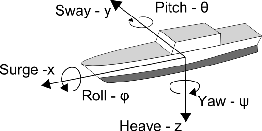
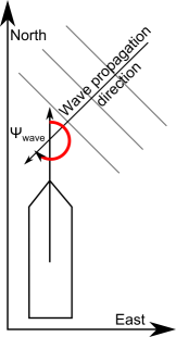
The vessels roll, pitch and yaw angles in the local coordinate system. The yaw angle is relative to the north direction. |
| QuaternionNED | 4 |
The rotation quaternion of the body as w,x,y,z |
| OmegaNED | 3 |
The rotational speed of the ship in the global "north-east-down" coordinate system |
| VelocityBody | 6 |
The full velocity vector of the vessel in body coordinates |
| BodyForce | 6 |
The total force acting on the vessel |
| FirstOrderWaveBody | 6 | The first order wave force, or froude-krylov force, as experienced in the body frame of the vessel The first order wave loads are defined as a sum of harmonic functions with the same frequency distribution as the wave elevation. |
| WaveDriftBody | 6 | The mean value of the higher order wave forces as experienced in the body frame of the vessel. The mean value of the heave, roll and pitch direction equals zero. |
| CrossFlowBody | 6 |
Cross flow are calculated by summation of section wise cross flow drag along the hull. Dampening in yaw is computed by calculating the moment contribution around the center of gravity for each sections cross flow drag force \[ v_r = v-x\cdot r\] \[ Y_{cross-flow} = -\frac{1}{2}\rho\int_{-Lpp/2}^{Lpp/2}T(x)C_d^2d(x)|v_r|v_r dx \] \[ N_{cross-flow} = -\frac{1}{2}\rho\int_{-Lpp/2}^{Lpp/2}T(x)\cdot x\cdot C_d^2d(x)|v_r|v_r dx \] |
| KineticEnergy | 1 |
The kinetic energy of the rigid body of the vessel |
| FluidEnergy | 1 |
The squared norm of the collection of fluid memory model states |
| SpeedInfo | 5 |
Information about the reference speeds in the potential data and the current speed of the vessel |
| Encounter | 5 |
Encounter frequency of the last wave in the sea environment list |
| CroiolisRigidBody | 6 |
Coriolis force of the rigid body mass and inertia tensors as formulated in the center of gravity |
| CroiolisFluidBody | 6 |
Coriolis force of the added mass and inertia tensors as formulated in the center of gravity |
| ViscousForceBody | 6 |
Viscous forces on body |
| SteadyStateBody | 6 |
Steady state control in BODY coordinates |
| SteadyStateNED | 6 |
Steady state control in NED coordinates |
| ResistanceBody | 6 | The calm water resistance of the hull in the surge direction The resistance force is the defined as the calm water resistance of the hull. The calm water resistance is divided into the Reynolds number ( \( R_n\)) dependent friction contribution, and the Froude number ( \( F_n\)) dependent wave generation from the flow pattern around the hull. The resistance is calculated by scaling the dimensional total resistance coefficient, \( C_{ts}\), by the wet surface, \( S\), on the current waterline. The total resistance coefficient is both \( R_n\) and \( F_n\) dependent and is defined as. |
| RotationForceFrame | 4 |
Rotation body if constrained to move parallel to the still ocean surface |
| RestoringForceBody | 6 |
The hydrostatic restoring force on the body |
| AdditionalDampeningBody | 6 |
The model supports additional user defined dampening forces. The forces are calculated from dimensionless dampening coefficients made dimensionless by \(m\) and by \(m\cdot L_{pp}\) for linear and rotational degrees of freedom respectively. The dampening force contains a linear and a quadratic modulus term which are controlled by separate dampening coefficients. \[ F = C_{d_linear} \cdot m \cdot v + C_{d_quadratic} \cdot m \cdot v|v|\] \[ M = C_{d_linear} \cdot m \cdot L_{pp} \cdot v + C_{d_quadratic} \cdot m \cdot L_{pp}\cdot v|v|\] The dampening force decreases with increasing forward velocity by weighting the force with \(exp{-\frac{1}{2}|U|}\) |
| FluidMemoryForceBody | 6 |
Fluid memory forces on body |
| RelativeVelocityBODY | 6 |
The relative velocity of the ship relative to the ambient (current) velocity |